&Notepad

Probabilistic Programming with Variational Inference:
Under the Hood

This note provides an introduction to probabilistic programming and variational inference using Pyro. The Pyro website also has a great tutorial, but it’s distinctly oriented more towards people with probability backgrounds than systems backgrounds. If you, like me, are good at software engineering and bad at probability (single-letter variables in particular), then this note is for you.

The pedagogy here is to use small code samples to run experiments that slowly build intuition for how the system works. The beauty of having a programming language, as opposed to learning from a probability textbook/class, is that we can turn questions into executable programs and see if reality matches our expectations. The ultimate goal is that you will have an end-to-end understanding of variational inference for simple probabilistic inference problems.

I highly recommend you follow along in a Jupyter notebook. Tweak parameters, ask questions, and stay engaged! You can use the notebook in the accompanying repository here: https://github.com/willcrichton/pyro-under-the-hood

Probabilistic programs and distributions

A probabilistic program is a program that samples from probability distributions. For example:

import pyro.distributions as dist
from pyro import sample
from torch import tensor

# A fair coin
coinflip = sample("coinflip", dist.Bernoulli(probs=0.5))
# e.g. coinflip == tensor(0.)

# A noisy sample
noisy_sample = sample("noisy_sample", dist.Normal(loc=0, scale=1))
# e.g. noisy_sample == tensor(0.35)

A probability distribution has two key functions: sample, which returns a single value in accordance with its probability (e.g. above, 0 and 1 are equally likely from the coin flip), and log_prob, which returns the log probability of a sample under the model.

Aside: Instead of doing dist.sample, we use sample(name, dist) for reasons you’ll see in a bit.

print(dist.Bernoulli(0.5).log_prob(tensor(0.)).exp()) # 0.5000
print(dist.Normal(0, 1).log_prob(tensor(0.35)).exp()) # 0.3752

By sampling from many distributions, we can describe a probabilistic generative model. As a running example, consider this sleep_model that describes the likely number of hours I’ll sleep on a given day. It generates a single data point by running the function top to bottom as a normal program.

def sleep_model():
    # Very likely to feel lazy
    feeling_lazy = sample("feeling_lazy", dist.Bernoulli(0.9))
    if feeling_lazy:
        # Only going to (possibly) ignore my alarm if I'm feeling lazy
        ignore_alarm = sample("ignore_alarm", dist.Bernoulli(0.8))
        # Will sleep more if I ignore my alarm
        amount_slept = sample("amount_slept",
                              dist.Normal(8 + 2 * ignore_alarm, 1))
    else:
        amount_slept = sample("amount_slept", dist.Normal(6, 1))
    return amount_slept

sleep_model() # e.g. 9.91
sleep_model() # e.g. 7.61
sleep_model() # e.g. 8.60

Aside: This is called a “generative” model because it has an explicit probabilistic model for every random variable (e.g. the prior on feeling_lazy). By contrast, a “discriminative” model only tries to model a conditional probabilistic distribution, where given some observations, you predict the distribution over unobserved variables.

At this point, our stochastic functions are nothing special, as in they do not need any specialized system or machinery to work. It’s mostly just normal Python. For example, we could implement one of these distributions ourselves:

from random import random

class Bernoulli:
    def __init__(self, p):
        self.p = p

    def sample(self):
        if random() < self.p:
            return tensor(1.)
        else:
            return tensor(0.)

    def log_prob(self, x):
        return (x * self.p + (1 - x) * (1 - self.p)).log()

b = Bernoulli(0.8)
b.sample() # e.g. 0.
b.log_prob(tensor(0.)).exp() # 0.2

Traces and conditioning

On the unconditional sleep model, we could ask a few questions, like:

• Joint probability of a sample: what is the probability that feeling_lazy = 1, ignore_alarm = 0, amount_slept = 10?
• Joint probability distribution: what is the probability for any possible assignment to all variables?
• Marginal probability of a sample: what is the probability that feeling_lazy is true?
• Marginal probability distribution: what is the probability over all values of amount_slept?

First, we need the ability to evaluate the probability of a joint assignment to each variable.

from pyro.poutine import trace
from pprint import pprint

# Runs the sleep model once and collects a trace
tr = trace(sleep_model).get_trace()

pprint({
    name: {
        'value': props['value'],
        'prob': props['fn'].log_prob(props['value']).exp()
    }
    for (name, props) in tr.nodes.items()
    if props['type'] == 'sample'
})
# {'amount_slept': {'prob': tensor(0.0799), 'value': tensor(8.2069)},
#  'feeling_lazy': {'prob': tensor(0.9000), 'value': tensor(1.)},
#  'ignore_alarm': {'prob': tensor(0.8000), 'value': tensor(1.)}}

print(tr.log_prob_sum().exp()) # 0.0575

Here, the trace feature will collect values every time they are sampled with sample and store them with the corresponding string name (that’s why we give each sample a name). With a little cleanup, we can print out the value and probability of each random variable’s value, along with the joint probability of the entire trace.

From a software engineering and PL perspective, the ability to do things like wrap a function with trace and collect its samples (called “effect handling”) is the core functionality of a probabilistic programming language like Pyro. Most of the remaining magic is in the automatic differentiation (in PyTorch) that we’ll see later. I highly recommend reading the Mini Pyro implementation to see how to design a modular effects system. For this note, it suffices to know that the sample mechanism enables an external entity calling the model function to observe and modify its execution.

The code above randomly generates a trace and shows its probability, but we want to compute the probability of a pre-selected set of values. For that, we can use condition:

from pyro import condition

cond_model = condition(sleep_model, {
    "feeling_lazy": tensor(1.),
    "ignore_alarm": tensor(0.),
    "amount_slept": tensor(10.)
})

trace(cond_model).get_trace().log_prob_sum().exp() # 0.0097

Here, condition means “force the sample to return the provided value, and compute the trace probability as if that value was sampled.” So for example, forcing feeling_lazy to 1 means the trace starts with probability 0.9. This also means the if statement will always go down the first branch. Inuitively, this particular choice should have low probability because if we didn’t ignore our alarm, then amount_slept should be closer to 8, not 10. That’s reflected in the low joint probability of 0.0097.

Now, we can produce an approximate answer to any of our questions above by sampling from the distribution enough times. For example, we can look at the marginal distribution over each variable:

import pandas as pd
import matplotlib.pyplot as plt

traces = []
for _ in range(1000):
    tr = trace(sleep_model).get_trace()
    values = {
        name: props['value'].item()
        for (name, props) in tr.nodes.items()
        if props['type'] == 'sample'
    }
    traces.append(values)

pd.DataFrame(traces).hist()

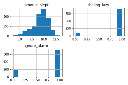
Look at each histogram and see if its distribution matches your expectations given the code for sleep_model. For example, the feeling_lazy histogram is true (or 1) about 90% of the time, which matches the prior belief Bernoulli(0.9).

Sampling conditional distributions

Here’s a few more questions we might want to answer.

• Given I slept 6 hours, what is the probability I was feeling lazy?
• What is the probability of me sleeping exactly 7.65 hours?

These are conditional probability questions, meaning they ask: given a particular value of some of the random variables, what are the likely values for the other random variables? The probability folk tend to call these “observed” and “latent” variables (often denoted by X and Z), respectively. A common use case for generative models is that the generated object is the thing you observe in the real world (like an image), and you want to guess the values of unobserved variables given that observation (like whether the image is a cat or a dog).

Aside: the second question is not obviously a conditional one. But to answer it, we need to compute $P(\text{feeling lazy}, \text{ignore alarm} \mid \text{amount slept})$. See my Pyro forum post for why.

For example, a smart watch can probably record my sleep patterns, but not record whether I was being lazy. So in the sleep model, we could say amount_slept is an observed random variable while feeling_lazy and ignore_alarm are latent random variables. Applying some basic probability theory, we can write out the quantity we want to compute:

Why did we rewrite the probability this way? Remember that with the unconditioned generative model, it’s easy for us to compute the probability of a joint assignment to every variable. So we can compute the probability of a single variable (a “marginal” probability), e.g. $P(\text{amount slept} = 6)$, as a sum over joint probabilities.

However, there are two problems with this approach. First, as the number of marginalized variables grows, we have an exponential increase in summation terms. In some cases, this issue can be addressed using algorithmic techniques like dynamic programming for variable elimination in the case of discrete variables. But the second issue is that for continuous variables, computing this marginal probability can quickly become intractable. For example, if feeling_lazy was a real-valued laziness score between 0 and 1 (presumably a more realistic model), then marginalizing that variable requires an integral instead of a sum. In general, producing an exact estimate of a conditional probability for a complex probabilistic program is not computationally feasible.

Approximate inference

The main idea is that instead of exactly computing the conditional probability distribution (or “posterior”) of interest, we can approximate it using a variety of techniques. Generally, these fall into two camps: sampling methods and variational methods. The CS 228 (Probabilistic Graphical Models at Stanford) course notes go in depth on both (sampling, variational). Essentially, for sampling methods, you use algorithms that continually draw samples from a changing probability distribution until eventually they converge on the true posterior of interest. The time to convergence is not known ahead of time. For variational methods, you use a simpler function that can be optimized to match the true posterior using standard optimization techniques like gradient descent.

How do you know which kind to use for a given probabilistic model? This StackOverflow answer highlights when it makes sense to use one vs. another (in summary: sampling for small data and when you really care about accuracy, variational otherwise). This note from Dustin Tran, a developer of the Edward PPL, highlights which kinds of inference PPLs beyond Pyro are generally used for.

As for Pyro, the introductory blog post and this PROBPROG’18 keynote provide a high-level motivation for Pyro’s focus on variational inference. One high-level theme is bringing Bayesian reasoning (i.e. quantifying uncertainty) to deep neural nets. Pyro’s integration with PyTorch is meant to facilitate the use of probabilistic programming techniques with standard neural nets. For example, one use case I heard of was using DNNs for 3D reconstruction from video, but augmenting the training process with probabilistic priors that use domain knowledge, e.g. if I’m reconstructing a stop sign, it should be close to an intersection.

That said, the space is still wide open, and researchers are working hard to develop new applications on top of these technologies. I recommend looking at the PROBPROG’18 talks to get a more general sense of PPL applications if you’re interested.

Variational inference 1: autodifferentiation

Since Pyro’s stake in the ground is on variational inference, let’s explore all the mechanics underneath it. For starters, we need to understand autodifferentiation, gradients, and backpropagation in PyTorch. Let’s say I have an extremely simple model that just samples a normal distribution with fixed parameters:

norm = dist.Normal(0, 1)
x = sample("x", norm)

However, let’s say I know the value of x = 5 and I want to find a mean $\mu$ to the normal distribution that maximizes the probability of seeing that x. For that, we can use a parameter:

from pyro import param

mu = param("mu", tensor(0.))
norm = dist.Normal(mu, 1)
x = sample("x", norm)

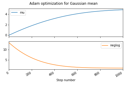
A parameter is a persistent value linked to a string name with an initial value here of 0. (It’s a Torch tensor with requires_grad=True.) Our goal is to update mu such that the probability of the value 5 under the normal distribution norm is maximized. PyTorch makes that quite easy:

prob = norm.log_prob(5)
print(prob, prob.exp()) # -13.4189, 0.000002

prob.backward() # Compute gradients with respect to probability

print(mu)      # 0.0
print(mu.grad) # 5.0
mu.data += mu.grad # Manually take gradient step

print(dist.Normal(mu, 1).log_prob(5)) # 0.3989

Make sure you understand what’s happening here. First, we compute the probability of 5 under the distribution $N(0, 1)$ which is expectedly quite small. The magic happens with prob.backward(). This essentially says: for each variable involved in computing the log probability, compute a delta (gradient) such that if moved by that delta, the log probability would increase. In this case, the gradient of 5 is the optimal solution to maximizing the probability of 5 under the model $N(5, 1)$, which has probability of 0.3989 as shown.

Note: this strategy assumes that all sampled distributions have differentiable log probability functions. Conveniently, this is true for every primitive distribution in the PyTorch standard library.

Next, let’s generalize this to the model/trace framework we used above.

def model():
    mu = param("mu", tensor(0.))
    return sample("x", dist.Normal(mu, 1))

cond_model = condition(model, {"x": 5})
tr = trace(cond_model).get_trace()
tr.log_prob_sum().backward()

mu = param("mu")
mu.data += mu.grad

This code is doing the exact same thing the previous block, but just less manually. When we condition the model, this asserts that x = 5 and adds N(mu, 1).log_prob(5) to the trace’s probability. Then running backpropagation will change the gradient on mu accordingly. This formulation is more general in that every sample location can contribute to the final log probability, and each parameter will be differentiated with respect to sum of all contributions.

The only remaining issue is the manual gradient steps. We currently both have to identify which parameters need to be updated, and then explicitly step them. PyTorch has a wide array of optimization algorithms that can do this for us, so we can just pick a common one like Adam.

from torch.optim import Adam

def model():
    mu = param("mu", tensor(0.))
    return sample("x", dist.Normal(mu, 1))

model() # Instantiate the mu parameter
cond_model = condition(model, {"x": 5})

# Large learning rate for demonstration purposes
optimizer = Adam([param("mu")], lr=0.01)
mus = []
losses = []
for _ in range(1000):
    tr = trace(cond_model).get_trace()

    # Optimizer wants to push positive values towards zero,
    # so use negative log probability
    prob = -tr.log_prob_sum()
    prob.backward()

    # Update parameters according to optimization strategy
    optimizer.step()

    # Zero all parameter gradients so they don't accumulate
    optimizer.zero_grad()

    # Record probability (or "loss") along with current mu
    losses.append(prob.item())
    mus.append(param("mu").item())

pd.DataFrame({"mu": mus, "loss": losses}).plot(subplots=True)

Variational inference 2: guide functions

To recap, we’ve seen now how to use autodifferentiation to optimize parameters to fit observations. Put another way, we implemented maximum likelihood learning, meaning we used optimization to find parameters that maximize the probability of data under our model. However, our goal was specifically to estimate the posterior distribution over unobserved (latent) variables. For example, returning to the sleep_model, let’s say we want to know the distribution over feeling_lazy and ignore_alarm if amount_slept = 6. Intuitively, although their prior likelihood is high, that amount of sleep is much more likely explained by not feeling lazy, so we would expect $P(fl, ia \mid as = 6)$ to be higher for $fl = ia = 0$. Ideally, that would be as simple as:

# Condition model on observed data
underslept = condition(sleep_model, {"amount_slept": 6.})

# Draw samples from conditioned model?
pd.Series(
  [trace(underslept).get_trace().nodes['feeling_lazy']['value'].item()
   for _ in range(100)]) \
  .hist()

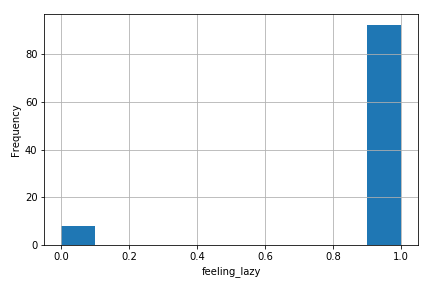
That doesn’t work! In fact, the histogram looks almost exactly like the prior on feeling_lazy. What we know so far should be enough to deduce why this doesn’t work—think about it for a second, and maybe revisit the explanation of condition above if you’re not sure.

Essentially, the condition only forces amount_slept to be 6 when we reach that point in the program, which only happens after we’ve sampled feeling_lazy and ignore_alarm. The condition has no way to exert influence opposite the flow of causality. (By contrast, if we conditioned on feeling_lazy = 1, then we could sample the model and it would work as intended!) This gets back to the intractability of computing a posterior, and why we’re using approximate methods.

For variational inference, the key idea is that we’re going to use a separate function from the model called the “guide” to represent the posterior. The guide is a stochastic function that represents a probability distribution over the latent (unobserved) variables. For example, this is a valid guide:

def sleep_guide():
  sample("feeling_lazy", dist.Delta(1.))
  sample("ignore_alarm", dist.Delta(0.))

trace(sleep_guide).get_trace().nodes['feeling_lazy']['value'] # 1.

The delta distribution assigns all probability to a single value, so the above guide has $P(fl = 1, ia = 0) = 1.0$ and all other assignments have zero probability.

Although this is a valid guide, it’s a bad one because its probability distribution is very different from the underslept model. (Although if we conditioned amount_slept = 8, it would be a decent guide!) How bad is this guide? In probability theory, it’s common to quantify the difference between two probability distributions through the KL divergence.

This essentially says: for all possible values of the latent variables, compute the difference in log probability between the model and the guide, and weight that difference by the likelihood of each assignment under the guide. In probability terms, you can think about that as an expectation of the difference in terms of the guide.

Note that the KL divergence is asymmetric, meaning $D_{KL}(p\|q) \neq D_{KL}(q\|p)$. That’s because the expression is an expectation in terms of either $p$ or $q$ (which ever function is on the left).

In order to compute $P_{\verb!model!}(fl, ia \mid as = 6)$, this still requires us to know $P_{\verb!model!}(as = 6)$ which is (in general) intractable due to marginalization as discussed above. Instead, we can apply a few transformations to factor out the intractable term and get a new expression called the “evidence lower bound” or ELBO:

The only difference is that the $P_{\verb!model!}$ term now is a joint probability instead of a conditional probability (and the overall term is not negated). See the Edward PPL page on $KL(q\|p)$ minimiazation for the gory details on how this works. We can compute this quantity in code:

def elbo(guide, cond_model):
  dist = 0.
  for fl in [0., 1.]:
    for ia in [0., 1.] if fl == 1. else [0.]:
      log_prob = lambda f: trace(condition(
        f, {"feeling_lazy": tensor(fl), "ignore_alarm": tensor(ia)})) \
        .get_trace().log_prob_sum()
      guide_prob = log_prob(guide)
      cond_model_prob = log_prob(cond_model)
      term = guide_prob.exp() * (cond_model_prob - guide_prob)
      if not torch.isnan(term):
        dist += term
  return dist

elbo(sleep_guide, underslept) # -4.63

Alright, well, that’s certainly a number. To check our intuition for how KL divergence works, we can also compare against a guide that has a probability distribution closer to our expected posterior.

def sleep_guide2():
  sample("feeling_lazy", dist.Delta(0.))
  sample("ignore_alarm", dist.Delta(0.))

elbo(sleep_guide2, underslept) # -3.22

As expected, the guide function with latent variables closer to our expected posterior has an ELBO closer to zero (meaning smaller KL divergence, meaning the distribution is closer to the actual posterior).

Variational inference 3: ELBO optimization

At last, we have reached the final step in variational inference: optimization. Specifically, our goal is to use the ELBO to determine how different the guide function is from our conditioned model, then use autodifferentiation to compute a gradient of the guide with respect to the ELBO. That is, we can know how to tweak the parameters of the guide function that lower the ELBO, or push it closer to the true conditioned probability distribution.

pyro.clear_param_store()

def sleep_guide():
    # Constraints ensure facts always remain true during optimization,
    # e.g. that the parameter of a Bernoulli is always between 0 and 1
    valid_prob = constraints.interval(0., 1.)
    fl_p = param('fl_p', tensor(0.8), constraint=valid_prob)
    ia_p = param('ia_p', tensor(0.9), constraint=valid_prob)
    feeling_lazy = sample('feeling_lazy', dist.Bernoulli(fl_p))

    # Consistent with the model, we only sample ignore_alarm if
    # feeling_lazy is true
    if feeling_lazy == 1.:
        sample('ignore_alarm', dist.Bernoulli(ia_p))

# Run once to register the param calls with Pyro
sleep_guide()

adam = Adam([param('fl_p').unconstrained(), param('ia_p').unconstrained()],
            lr=0.005, betas=(0.90, 0.999))
param_vals = []

for _ in range(2000):
    # We can use our elbo function from earlier and compute its gradient
    loss = -elbo(sleep_guide, underslept)
    loss.backward()

    adam.step()
    adam.zero_grad()

    param_vals.append({k: param(k).item() for k in ['fl_p', 'ia_p']})

pd.DataFrame(param_vals).plot(subplots=True)

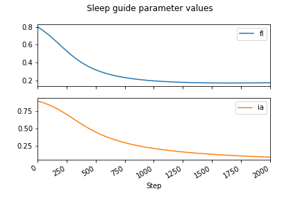
Perfect! This plot reflects our belief that the probability of feeling lazy should be lower if the observed amount slept is low. Our sleep_guide now properly represents (an approximation to) the posterior $P(fl, ia \mid as = 6)$. Carefully observe that the parameter fl_p is distinct from the random variable feeling_lazy. That is, fl_p is a deterministic value (not sampled from a distribution) that changes during optimization, and is a parameter to the Bernoulli distribution describing how feeling_lazy is sampled.

However, there’s two nagging questions left: what if feeling_lazy was real-valued (as opposed to 0 or 1)? And how did we come up with this guide function? As mentioned in the “Approximate inference” section, if feeling_lazy was a score (real-valued, say between 0 and 1), then we would have to change our elbo function to reflect that.

def elbo(guide, cond_model):
  dist = 0.
  for fl in (every value between 0 and 1):
    ...
  return dist

Again we return to “computationally intractable”. We’re essentially computing an integral, which we can either do analytically (compute a closed form for the ELBO that doesn’t have an integral in it), or approximately (pick a few values between 0 and 1, and approximate the integral with an average). The simplest approximation only uses a single random assignment to the latent variables.

from pyro.poutine import replay

def elbo_approx(guide, cond_model):
    guide_trace = trace(guide).get_trace()
    model_trace = trace(replay(cond_model, guide_trace)).get_trace()
    return model_trace.log_prob_sum() - guide_trace.log_prob_sum()

Rather than simulate the guide and model under every assignment to the latents, we instead sample the guide for a single assignment to feeling_lazy and ignore_alarm (contained in guide_trace). We then condition the model on that assignment (replay is exactly like condition except it takes as input a trace object instead of a dictionary), and compare the probability of the model’s trace versus the guide’s trace. Again, this is approximating the expectation with a single assignment drawn from the guide’s distribution.

We can directly replace our elbo with elbo_approx in the optimization code from earlier, and see how it works:

for _ in range(2000):
    loss = -elbo_approx(sleep_guide, underslept)
    loss.backward()
    adam.step()
    adam.zero_grad()

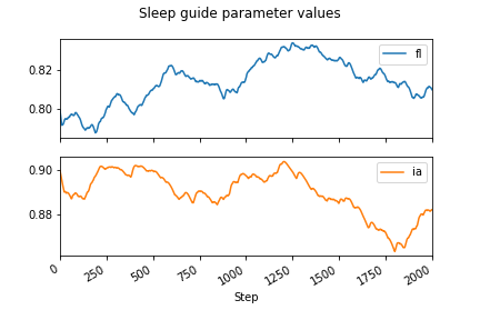
Oh no! That didn’t work at all. The optimization seems to just have randomly moved the parameters around, not reduced them to 0 as we expected from earlier. To get an intuition for why this didn’t work, we can look at the value of the gradient on the fl parameter.

grad_vals = []
for _ in range(2000):
    loss = -elbo_approx(sleep_guide, underslept)
    loss.backward()
    grad_vals.append(param('fl').unconstrained().grad.item())
    ...

pd.Series(grad_vals).plot()

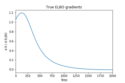
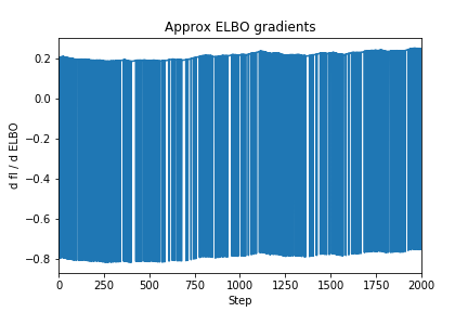
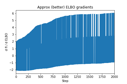
As you can see, the gradient of the true ELBO is much smoother (lower variance), since it considers every possible latent variable assignment instead of just one. Intuitively, the reason for this variance is that the output (or “support”) of the Bernoulli distribution is discrete, i.e. true/false or 1/0. So the probability of one sample to the next can be drastically different, e.g. if $X \sim \text{Bernoulli(0.8)}$ then $P(X = 0) = 0.2$ and $P(X = 1) = 0.8$, so $P(X = 1) - P(X = 0) = 0.6$. By contrast, if we’re sampling a normal distribution which has many more possible outputs, a pair of samples will likely have a smaller difference in probability.

So how do we solve this? Well, in general, dealing with tricky gradient issues is just one of the hard parts of variational inference. The Pyro SVI tutorial discusses a few approaches, which I personally could follow mechanically, but I still don’t really get the intuition behind why they work.

I’ve read several blog posts about this gradient issue, but they always just seem to derive lots of formulas without really delving into the “why”… so if you have a good explanation, please let me know!

In this specific case, it turns out that a good tool is to replace the actual ELBO with a “surrogate” objective that yields more stable gradients for our problem (again, see Pyro docs for discussion).

def elbo_better_approx(guide, cond_model):
    guide_trace = trace(guide).get_trace()
    model_trace = trace(replay(cond_model, guide_trace)).get_trace()
    elbo = model_trace.log_prob_sum() - guide_trace.log_prob_sum()
    # "detach" means "don't compute gradients through this expression"
    return guide_trace.log_prob_sum() * elbo.detach() + elbo

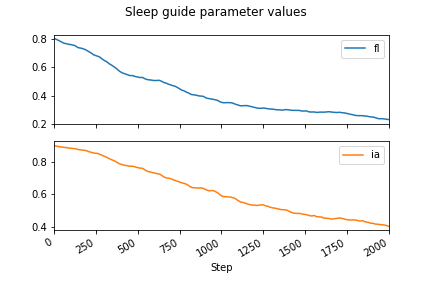
Optimizing with respect to this objective yields much better results:

To bring this back full circle, the hand-crafted variational inference above does (roughly) the same thing as this high-level Pyro code:

from pyro.optim import Adam
from pyro.infer import SVI, Trace_ELBO

adam = Adam({"lr": 0.005, "betas": (0.90, 0.999)})
svi = SVI(underslept, sleep_guide, adam, loss=Trace_ELBO())

param_vals = []
for _ in range(2000):
    svi.step()
    param_vals.append({k: param(k).item() for k in ["fl", "ia"]})

pd.DataFrame(param_vals).plot(subplots=True)

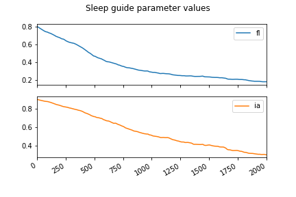
The SVI object is responsible for collecting the different param objects and calling loss.backward(), adam.step(), and zeroing the gradients. See the Mini Pyro implementation for how you could implement this object yourself. The Trace_ELBO object is similar to our elbo_better_approx except with a few more tricks for dealing with conditional independence in models (see the Pyro docs for more on that).

At this point, you should be able to read the above Pyro code and know (almost) exactly what’s going on under the hood. Similar to knowing what happens when you Google search, you should know what happens when you svi.step(). To recap:

• The goal is to take a model conditioned on observations, and produce a new function whose distribution over the unobserved variables is the same as the conditioned model.
• The core process is to use a guide function containing parameters that are optimized with respect to the ELBO, a measure of the difference between the guide and the model.
• We use Torch’s autodifferentiation to compute the gradient of the parameters with respect to the ELBO.
• We approximate the true ELBO with individual samples, and use a bag of tricks to rewrite our approximate ELBO in a way that produces more stable gradients.

As an exercise for the reader: we never technically answered our question, what is the probability of feeling lazy given that I slept for 6 hours? Think about how you could use the optimized sleep_guide to come up with an answer.

Addendum: guide design

A still-looming question is: how did we choose our guide? I just kind of asserted that we would use the one we did. As the Pyro docs state:

The guide function should generally be chosen so that, in principle, it is flexible enough to closely approximate the distribution over all unobserved sample statements in the model.

In general, guide design seems to be something of a dark art. One basic principle is that parameters should be continuous to permit iterative optimization through gradient descent. For example, if we use a sleep guide that just uses delta distributions on boolean parameters:

def sleep_guide_delta():
    is_bool = constraints.boolean
    fl = param('fl', tensor(1.0), constraint=is_bool)
    ia = param('ia', tensor(0.0), constraint=is_bool)
    feeling_lazy = sample("feeling_lazy", dist.Delta(fl))
    if feeling_lazy == 1.0:
        sample("ignore_alarm", dist.Delta(ia))

svi = SVI(underslept, sleep_guide_delta, adam, loss=Trace_ELBO())
svi.step() # NotImplementedError: Cannot transform _Boolean constraints

It seems like Pyro’s VI can’t handle that case at all. But beyond that, you just experiment with different guides, run your optimization, and see what ends up closest to the desired posterior (according to the ELBO). Given the relative nascency of probabilistic programming, this seems like an active area of investigation and research. Some recent work has focused on automatically deriving guide functions, as implemented in the pyro.contrib.autoguide module. Your best bet is probably just to learn from the litany of examples in the Pyro repo.

That’s all for now. I hope that you’ve found this extended exploration through the Pyro internals useful in concretizing your understanding of how probabilistic programming with variational inference works. If you’re interested in better understanding the types of problems PPLs can be used for, I encourage you to look at the Forest DB repository of probabilistic programs, skim the PROBPROG’18 proceedings for reports from academia and industry, or read through Probabilistic Models of Cognition to see applications of PPLs to cognitive psychology.