$$
% Typography and symbols
\newcommand{\msf}[1]{\mathsf{#1}}
\newcommand{\ctx}{\Gamma}
\newcommand{\qamp}{&\quad}
\newcommand{\qqamp}{&&\quad}
\newcommand{\Coloneqq}{::=}
\newcommand{\proves}{\vdash}
\newcommand{\star}[1]{#1^{*}}
\newcommand{\eps}{\varepsilon}
\newcommand{\nul}{\varnothing}
\newcommand{\brc}[1]{\{{#1}\}}
\newcommand{\binopm}[2]{#1~\bar{\oplus}~#2}
\newcommand{\mag}[1]{|{#1}|}
\newcommand{\aequiv}{\equiv_\alpha}
\newcommand{\semi}[2]{{#1};~{#2}}
% Untyped lambda calculus
\newcommand{\fun}[2]{\lambda ~ {#1} ~ . ~ {#2}}
\newcommand{\app}[2]{#1 ~ #2}
\newcommand{\fix}[3]{\msf{fix}~({#1} : {#2}) ~ . ~ #3 }
\newcommand{\truet}{\msf{true}}
\newcommand{\falset}{\msf{false}}
\newcommand{\define}[2]{{#1} \triangleq {#2}}
% Typed lambda calculus - expressions
\newcommand{\funt}[3]{\lambda ~ \left(#1 : #2\right) ~ . ~ #3}
\newcommand{\lett}[4]{\msf{let} ~ \hasType{#1}{#2} = #3 ~ \msf{in} ~ #4}
\newcommand{\letrec}[4]{\msf{letrec} ~ \hasType{#1}{#2} = #3 ~ \msf{in} ~ #4}a
\newcommand{\ift}[3]{\msf{if} ~ {#1} ~ \msf{then} ~ {#2} ~ \msf{else} ~ {#3}}
\newcommand{\rec}[5]{\msf{rec}(#1; ~ #2.#3.#4)(#5)}
\newcommand{\case}[5]{\msf{case} ~ {#1} ~ \{ L(#2) \to #3 \mid R(#4) \to #5 \}}
\newcommand{\pair}[2]{\left({#1},~{#2}\right)}
\newcommand{\proj}[2]{#1 . #2}
\newcommand{\inj}[3]{\msf{inj} ~ #1 = #2 ~ \msf{as} ~ #3}
\newcommand{\letv}[3]{\msf{let} ~ {#1} = {#2} ~ \msf{in} ~ {#3}}
\newcommand{\fold}[2]{\msf{fold}~{#1}~\msf{as}~{#2}}
\newcommand{\unfold}[1]{\msf{unfold}~{#1}}
\newcommand{\poly}[2]{\Lambda~{#1}~.~ #2}
\newcommand{\polyapp}[2]{{#1}~\left[{#2}\right]}
\newcommand{\export}[3]{\msf{export}~ #1 ~\msf{without}~{#2}~\msf{as}~ #3}
\newcommand{\import}[4]{\msf{import} ~ ({#1}, {#2}) = {#3} ~ \msf{in} ~ #4}
% Typed lambda calculus - types
\newcommand{\tnum}{\msf{num}}
\newcommand{\tstr}{\msf{string}}
\newcommand{\tint}{\msf{int}}
\newcommand{\tbool}{\msf{bool}}
\newcommand{\tfun}[2]{#1 \rightarrow #2}
\newcommand{\tprod}[2]{#1 \times #2}
\newcommand{\tsum}[2]{#1 + #2}
\newcommand{\trec}[2]{\mu~{#1}~.~{#2}}
\newcommand{\tvoid}{\msf{void}}
\newcommand{\tunit}{\msf{unit}}
\newcommand{\tpoly}[2]{\forall~{#1}~.~{#2}}
\newcommand{\tmod}[2]{\exists ~ {#1} ~ . ~ #2}
% WebAssembly
\newcommand{\wconst}[1]{\msf{i32.const}~{#1}}
\newcommand{\wbinop}[1]{\msf{i32}.{#1}}
\newcommand{\wgetlocal}[1]{\msf{get\_local}~{#1}}
\newcommand{\wsetlocal}[1]{\msf{set\_local}~{#1}}
\newcommand{\wgetglobal}[1]{\msf{get\_global}~{#1}}
\newcommand{\wsetglobal}[1]{\msf{set\_global}~{#1}}
\newcommand{\wload}{\msf{i32.load}}
\newcommand{\wstore}{\msf{i32.store}}
\newcommand{\wsize}{\msf{memory.size}}
\newcommand{\wgrow}{\msf{memory.grow}}
\newcommand{\wunreachable}{\msf{unreachable}}
\newcommand{\wblock}[1]{\msf{block}~{#1}}
\newcommand{\wloop}[1]{\msf{loop}~{#1}}
\newcommand{\wbr}[1]{\msf{br}~{#1}}
\newcommand{\wbrif}[1]{\msf{br\_if}~{#1}}
\newcommand{\wreturn}{\msf{return}}
\newcommand{\wcall}[1]{\msf{call}~{#1}}
\newcommand{\wlabel}[2]{\msf{label}~\{#1\}~{#2}}
\newcommand{\wframe}[2]{\msf{frame}~({#1}, {#2})}
\newcommand{\wtrapping}{\msf{trapping}}
\newcommand{\wbreaking}[1]{\msf{breaking}~{#1}}
\newcommand{\wreturning}[1]{\msf{returning}~{#1}}
\newcommand{\wconfig}[5]{\{\msf{module}{:}~{#1};~\msf{mem}{:}~{#2};~\msf{locals}{:}~{#3};~\msf{stack}{:}~{#4};~\msf{instrs}{:}~{#5}\}}
\newcommand{\wfunc}[4]{\{\msf{params}{:}~{#1};~\msf{locals}{:}~{#2};~\msf{return}~{#3};~\msf{body}{:}~{#4}\}}
\newcommand{\wmodule}[1]{\{\msf{funcs}{:}~{#1}\}}
\newcommand{\wcg}{\msf{globals}}
\newcommand{\wcf}{\msf{funcs}}
\newcommand{\wci}{\msf{instrs}}
\newcommand{\wcs}{\msf{stack}}
\newcommand{\wcl}{\msf{locals}}
\newcommand{\wclab}{\msf{labels}}
\newcommand{\wcm}{\msf{mem}}
\newcommand{\wcmod}{\msf{module}}
\newcommand{\wsteps}[2]{\steps{\brc{#1}}{\brc{#2}}}
\newcommand{\with}{\underline{\msf{with}}}
\newcommand{\wvalid}[2]{{#1} \vdash {#2}~\msf{valid}}
\newcommand{\wif}[2]{\msf{if}~{#1}~{\msf{else}}~{#2}}
\newcommand{\wfor}[4]{\msf{for}~(\msf{init}~{#1})~(\msf{cond}~{#2})~(\msf{post}~{#3})~{#4}}
% assign4.3 custom
\newcommand{\wtry}[2]{\msf{try}~{#1}~\msf{catch}~{#2}}
\newcommand{\wraise}{\msf{raise}}
\newcommand{\wraising}[1]{\msf{raising}~{#1}}
\newcommand{\wconst}[1]{\msf{i32.const}~{#1}}
\newcommand{\wbinop}[1]{\msf{i32}.{#1}}
\newcommand{\wgetlocal}[1]{\msf{get\_local}~{#1}}
\newcommand{\wsetlocal}[1]{\msf{set\_local}~{#1}}
\newcommand{\wgetglobal}[1]{\msf{get\_global}~{#1}}
\newcommand{\wsetglobal}[1]{\msf{set\_global}~{#1}}
\newcommand{\wload}{\msf{i32.load}}
\newcommand{\wstore}{\msf{i32.store}}
\newcommand{\wsize}{\msf{memory.size}}
\newcommand{\wgrow}{\msf{memory.grow}}
\newcommand{\wunreachable}{\msf{unreachable}}
\newcommand{\wblock}[1]{\msf{block}~{#1}}
\newcommand{\wloop}[1]{\msf{loop}~{#1}}
\newcommand{\wbr}[1]{\msf{br}~{#1}}
\newcommand{\wbrif}[1]{\msf{br\_if}~{#1}}
\newcommand{\wreturn}{\msf{return}}
\newcommand{\wcall}[1]{\msf{call}~{#1}}
\newcommand{\wlabel}[2]{\msf{label}~\{#1\}~{#2}}
\newcommand{\wframe}[2]{\msf{frame}~({#1}, {#2})}
\newcommand{\wtrapping}{\msf{trapping}}
\newcommand{\wbreaking}[1]{\msf{breaking}~{#1}}
\newcommand{\wreturning}[1]{\msf{returning}~{#1}}
\newcommand{\wconfig}[5]{\{\msf{module}{:}~{#1};~\msf{mem}{:}~{#2};~\msf{locals}{:}~{#3};~\msf{stack}{:}~{#4};~\msf{instrs}{:}~{#5}\}}
\newcommand{\wfunc}[4]{\{\msf{params}{:}~{#1};~\msf{locals}{:}~{#2};~\msf{return}~{#3};~\msf{body}{:}~{#4}\}}
\newcommand{\wmodule}[1]{\{\msf{funcs}{:}~{#1}\}}
\newcommand{\wcg}{\msf{globals}}
\newcommand{\wcf}{\msf{funcs}}
\newcommand{\wci}{\msf{instrs}}
\newcommand{\wcs}{\msf{stack}}
\newcommand{\wcl}{\msf{locals}}
\newcommand{\wcm}{\msf{mem}}
\newcommand{\wcmod}{\msf{module}}
\newcommand{\wsteps}[2]{\steps{\brc{#1}}{\brc{#2}}}
\newcommand{\with}{\underline{\msf{with}}}
\newcommand{\wvalid}[2]{{#1} \vdash {#2}~\msf{valid}}
% assign4.3 custom
\newcommand{\wtry}[2]{\msf{try}~{#1}~\msf{catch}~{#2}}
\newcommand{\wraise}{\msf{raise}}
\newcommand{\wraising}[1]{\msf{raising}~{#1}}
\newcommand{\wif}[2]{\msf{if}~{#1}~{\msf{else}}~{#2}}
\newcommand{\wfor}[4]{\msf{for}~(\msf{init}~{#1})~(\msf{cond}~{#2})~(\msf{post}~{#3})~{#4}}
\newcommand{\windirect}[1]{\msf{call\_indirect}~{#1}}
% session types
\newcommand{\ssend}[2]{\msf{send}~{#1};~{#2}}
\newcommand{\srecv}[2]{\msf{recv}~{#1};~{#2}}
\newcommand{\soffer}[4]{\msf{offer}~\{{#1}\colon({#2})\mid{#3}\colon({#4})\}}
\newcommand{\schoose}[4]{\msf{choose}~\{{#1}\colon({#2})\mid{#3}\colon({#4})\}}
\newcommand{\srec}[1]{\msf{label};~{#1}}
\newcommand{\sgoto}[1]{\msf{goto}~{#1}}
\newcommand{\dual}[1]{\overline{#1}}
% Inference rules
\newcommand{\inferrule}[3][]{\cfrac{#2}{#3}\;{#1}}
\newcommand{\ir}[3]{\inferrule[\text{(#1)}]{#2}{#3}}
\newcommand{\s}{\hspace{1em}}
\newcommand{\nl}{\\[2em]}
\newcommand{\evalto}{\boldsymbol{\overset{*}{\mapsto}}}
\newcommand{\steps}[2]{#1 \boldsymbol{\mapsto} #2}
\newcommand{\evals}[2]{#1 \evalto #2}
\newcommand{\subst}[3]{[#1 \rightarrow #2] ~ #3}
\newcommand{\dynJ}[2]{#1 \proves #2}
\newcommand{\dynJC}[1]{\dynJ{\ctx}{#1}}
\newcommand{\typeJ}[3]{#1 \proves \hasType{#2}{#3}}
\newcommand{\typeJC}[2]{\typeJ{\ctx}{#1}{#2}}
\newcommand{\hasType}[2]{#1 : #2}
\newcommand{\val}[1]{#1~\msf{val}}
\newcommand{\num}[1]{\msf{Int}(#1)}
\newcommand{\err}[1]{#1~\msf{err}}
\newcommand{\trans}[2]{#1 \leadsto #2}
\newcommand{\size}[1]{\left|#1\right|}
$$
Programming in the Debugger
Will Crichton
—
April 20, 2018
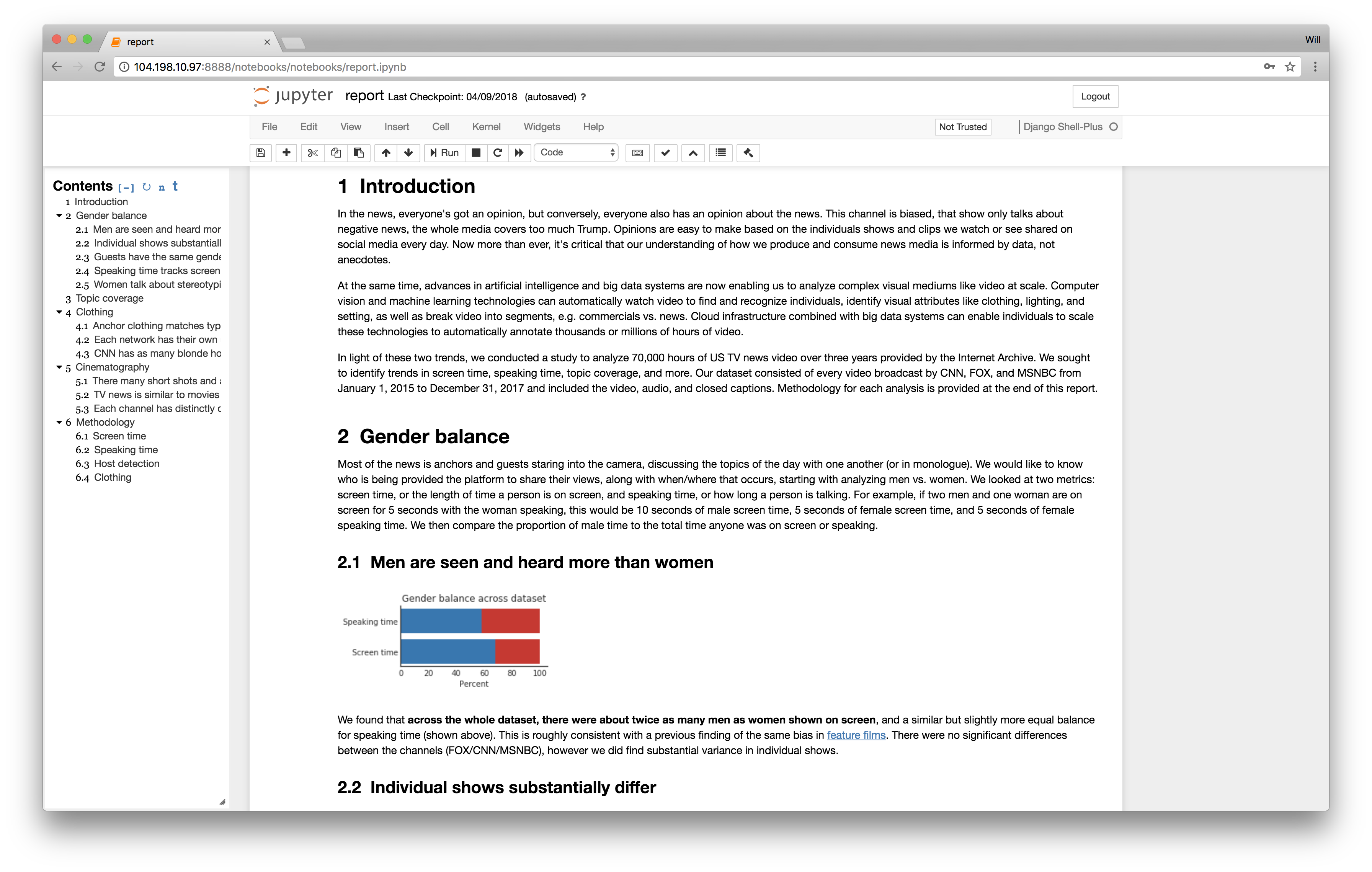
Jupyter presents a unique programming style where the programmer can change her code while it's running, reducing the cost of mistakes and improving the interactivity of the programming process. I discuss the benefits and limitations of this approach along with the related work.
For the last year, I’ve been creating a lot of programs for data manipulation (specifically video analysis), and while the heavy lifting is usually in C or Rust, the lighter-weight metadata processing is all Python. As with many in the data science field, I’ve fallen in love with Jupyter notebooks, the code editing and output visualization environment. Jupyter’s most-touted feature is the ability to intertwine code, narrative, and visualization. Write code to create a graph and display it inline. Create literate documents with Markdown headers. And this is great! I love the ability to create living documents that change when your data does, like the one below I’ve been developing.
However, after using Jupyter for a while, I’ve noticed that it has changed my programming process in a way more fundamental than simply inlining visualization of results. Specifically, Jupyter enables programmers to edit their program while it is running. Here’s a quick example. Let’s say I have some expensive computation (detect faces in a video) and I want to post-process the results (draw boxes on the faces). Normally, the development process would be, I write a first draft of the program:
## face.py

# Takes 1 minute
video = load_video()

# Takes 20 minutes
all_faces = detect_faces(video)

# Takes 1 minute
for (frame, frame_faces) in zip(video.frames(), all_faces):
    cv2.imwrite('frame{}.jpg', draw_faces(frame, frame_faces))
If I run this program (python face.py), it would probably run to completion, except… oh no! A bug: I forgot to format the 'frame{}.jpg' string (note: not a bug a type system would have found, this isn’t just a dynamic typing issue). But I had to wait 22 minutes to discover this bug, and now when I fix it, I have to re-run my program and wait another 22 minutes to confirm that it works. Why? Even though the bug was in the post-processing, I have to re-run the core computation, since my program exited upon completion, releasing its contents from memory. I should be able to just change the bug, and verify my change in only a minute. How can we do that?
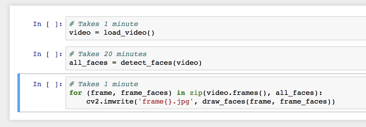
Consider the same workflow, but running in Jupyter. First, I would define a separate code cell to run each part of the pipeline:
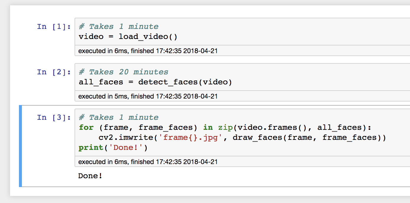
I would execute each part of the pipeline:
Then, after inspecting the output and noticing the error, change the last code cell, and only re-run that cell:
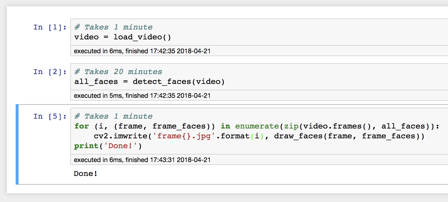
This works exactly as intended! We were able to edit our program while it was running, and then re-run only the part that needed fixing. In some sense, this is an obvious result—a REPL is designed to do exactly this, allow you to create new code while inside a long-running programming environment. But the difference between Jupyter and a REPL is that Jupyter is persistent. Code which I write in a REPL disappears along with my data when the REPL exits, but Jupyter notebooks hang around. Jupyter’s structure of delimited code cells enables a programming style where each can be treated like an atomic unit, where if it completes, then its effects are persisted in memory for other code cells to process.
More generally, we can view this as a form of programming in the debugger. Rather than separating code creation and code execution as different phases of the programming cycle, they become intertwined. Jupyter performs the many functions of a debugger—inspecting the values of variables, setting breakpoints (ends of code cells), providing rich visualization of program intermediates (e.g. graphs)—except the programmer can react to program’s execution by changing the code while it runs.
However, this style of programming with Jupyter has its limits. For example, Jupyter penalizes abstraction by removing this interactive debuggability. In the face detection example above, if we made our code generic over the input video:
def detect_and_draw_faces(video)
    all_faces = detect_faces(video)
    for (frame, frame_faces) in zip(video.frames(), all_faces):
        cv2.imwrite('frame{}.jpg', draw_faces(frame, frame_faces))

video = load_video()
detect_and_draw_faces(video)
Because a single function cannot be split up over multiple code cells, we cannot break the execution of the function in the middle, change its code, and continue to run. Interactive editing and debugging is limited to top-level code. This is actually a really common problem for me, since I’ll write straight-line code for a single instance of the pipeline (on a particular video, as originally), but then want to run it over many videos in batch. However, inevitably I missed some edge case not exposed by the example video, but I can no longer debug the issue in the same way.
Additionally, this model of debugging/editing only works for code blocks that are pure, i.e. don’t rely on global state outside the block. For example, if I have a program like:
x = 0

### new code block ###

x += 1
print('{}'.format(y))
Then if I fix the variable name error (format(x) instead of y) and re-run the code block, the value of x has changed, and my program output depends on the number of times I debugged the function. Not good! Essentially we need some kind of reverse debugging (also time-traveling debugging), where we can rewind the state of the program back to a reasonable point before the error occured. This has been done for Python, but to my knowledge has never been integrated into Jupyter in a sensible way.
This idea has existed in many other forms, particularly in the web world where hot-swapping code is common. An ideal model is embodied in the Elm Reactor time-traveling debugger for the Elm programming language. If your language is pure and functionally reactive, then you almost get this mode of debugging for free (plus a little tooling). The interesting question, then, is if your language is impure, or if your language gradually ensured purity, how far can we go with these edit/debug interactions? Could we integrate reverse debugging into Jupyter for Python? Could I edit a function in the middle of its execution? In what scenarios would such a programming style be most useful?
As always, let me know what you think. Either drop me a line at wcrichto@cs.stanford.edu or leave a comment on the Hacker News thread.